Transport Calculations (Oxygen version)

 

by Maria Troppenz & Santiago Rigamonti for exciting oxygen

Purpose: In this tutorial you will learn how to calculate electronic transport coefficients with exciting. The coefficients are obtained by solving the linearized Boltzmann equation in the constant relaxation time approximation. They are calculated for bulk silicon.

Fold Table of Contents 0. Define relevant environment variables 1. Theoretical background 2. Transport coefficients of Bulk Silicon i) Preparation of the calculation ii) Calculation of the transport coefficients at room temperature iii) Calculation of the transport coefficients at different doping concentrations

---

0. Define relevant environment variables

Read the following paragraphs before starting with the rest of this tutorial!

Before starting, be sure that relevant environment variables are already defined as specified in How to set environment variables for tutorials scripts. The following script is used in this tutorial:

• PLOT-files.py: Python visualization tool for multiple files with the same name in different directories (for more details, see The python script "PLOT-files.py").

From now on the symbol $ will indicate the shell prompt.

Important note: All input parameters are in atomic units!

---

1. Theoretical background

---

☛ Transport coefficients by using the Boltzmann equation

---

2. Transport coefficients of Bulk Silicon

To start the tutorial, create a new, empty directory named BE-Si and move into it.

$ mkdir BE-Si
$ cd BE-Si

i) Preparation of the calculation

Save the following lines as input.xml:

<input>
   <title>Bulk Silicon</title>
   <structure speciespath="$EXCITINGROOT/species/">
      <crystal scale="10.26">
         <basevect>0.0   0.5   0.5</basevect>
         <basevect>0.5   0.0   0.5</basevect>
         <basevect>0.5   0.5   0.0</basevect>
      </crystal>
      <species speciesfile="Si.xml">
         <atom coord="0.00  0.00  0.00"></atom>
         <atom coord="0.25  0.25  0.25"></atom>
      </species>
   </structure>
   <groundstate
      do="fromscratch"
      xctype="GGA_PBE_SOL"
      ngridk="4 4 4"
      rgkmax="8.0"
      gmaxvr="14.0"
      maxscl="100">
   </groundstate>
</input>

Set up $EXCITINGROOT to the correct root directory in speciespath and execute exciting_smp with the commands

$ SETUP-excitingroot.sh
$ time exciting_smp

To gain a better understanding of the later calculated transport coefficients of silicon, you may want to look at the band structure. For this, please expand the link below and follow the instructions.

---

☛ Calculation of the bandstructure of bulk silicon

---

ii) Calculation of the transport coefficients at room temperature

In the following, we calculate the transport coefficients with respect to the chemical potential at a constant temperature (here 300K). The equations of the transport coefficients (see Section 1) contain the derivative of the Fermi distribution function f0. That means that only k-points with eigenenergies near the Fermi surface contribute to the coefficients. In order to achieve a sufficient representation of the energy bands in this area, a fine k-grid is needed.

To obtain eigenenergies for a fine k-grid, we perform a single self-consistency loop on top of the previous ground-state calculation by changing in input.xml

• the attribute do = "fromfile";
• the attribute ngridk = "40 40 40";
• the attribute maxscl = "1";

in the element groundstate (for more details see Input Reference).

The element groundstate in input.xml should now look like this:

...
   <groundstate
      do="fromfile"
      xctype="GGA_PBE_SOL"
      ngridk="40 40 40"
      rgkmax="8.0"
      gmaxvr="14.0"
      maxscl="1">
   </groundstate>
...

In order to calculate the transport coefficients, delete in your input.xml the "old" properties block that you used for calculating the electronic band-structure:

   <properties>
 
      <bandstructure>
         ...
      </bandstructure>
 
   </properties>

and substitute it with

   <properties>
 
      <momentummatrix/>
      <boltzequ
         energyReference="efermi"
         transportDfRange="-0.5 0.5"
         transportDfSpacing="0.001"
         temperatureRange="300 300"
         temperatureSpacing="1"
         chemicalPotentialRange="-0.05 0.05"
         chemicalPotentialSpacing="0.0001"
         evOutputEnergies="true"
         siOutputUnits="true">
         <etCoeffComponents>1 1</etCoeffComponents>
         <etCoeffComponents>2 2</etCoeffComponents>
         <etCoeffComponents>3 3</etCoeffComponents>     
      </boltzequ>
 
   </properties>

With inserting the element momentummatrix, the momentum matrix elements are calculated. Inside the element boltzequ, you define the attributes needed for the calculation of the transport coefficients.

An explanation of the attributes can be found by expanding the link below or in Input Reference.

---

☛ Table of the attributes used for the transport coefficients

---

By executing exciting_smp

$ time exciting_smp

the Seebeck coefficient S, the electrical conductivity over the relaxation time σ/τ, and the thermal conductivity over the relaxation time κ0/τ are calculated for the temperature range and chemical potential range defined in input.xml. They are found in the files SEEBECK_COMP.OUT, ELECTCOND_COMP.OUT, and THERMALCOND_COMP.OUT, respectively, where COMP denotes the tensor component specified by the integer pair given in condcomp. Furthermore, the figure of merit estimated by Z=(σS2/κ0) can be found in file Z_COMP.OUT.

Please note: σ and κ0 are not directly given, but the output files contain the coefficients σ/τ and κ0/τ. τ itself is constant (does not depend on electronic structure with kk and n), and can be multiplied afterwards.

Now, the transport coefficients are calculated and you can plot them by using PLOT-files.py. A detailed description of this plot script can be found in The Python Script PLOT-files.py.

The Seebeck coefficient at the temperature of 300K can be visualized with the following commands:

$ cp SEEBECK_11.OUT S11
$ cp SEEBECK_22.OUT S22
$ cp SEEBECK_33.OUT S33
$ PLOT-files.py -f S11 S22 S33  -cx 2  -cy 3  -ll '$S_{xx}$' '$S_{yy}$' '$S_{zz}$'  -x -1 1  -lx '$\mu$ [eV]'  -ly 'S [$\mu$V/K]'  -ys 1e6  -rp

The output is saved in PLOT.png and PLOT.eps, and looks as follows:

Assuming a relaxation time τ of 10 fs, the electrical conductivity can be obtained as:

$ cp ELECTCOND_11.OUT E11
$ cp ELECTCOND_22.OUT E22
$ cp ELECTCOND_33.OUT E33
$ PLOT-files.py -f E11 E22 E33  -cx 2  -cy 3  -ll '$\sigma_{xx}$' '$\sigma_{yy}$' '$\sigma_{zz}$'  -x -0.5 0.5  -y 0 9000  -lx '$\mu$ [eV]'  -ly '$\sigma$ [S/cm]'  -ys 1e-16  -lp 'upper center'  -rp  -mty 5

Output:

And the corresponding power factor looks as:

$ paste ELECTCOND_11.OUT SEEBECK_11.OUT | awk '{ printf $1 "\t" $2 "\t" $3*$7*$7 "\n" }' > PF11
$ paste ELECTCOND_22.OUT SEEBECK_22.OUT | awk '{ printf $1 "\t" $2 "\t" $3*$7*$7 "\n" }' > PF22
$ paste ELECTCOND_33.OUT SEEBECK_33.OUT | awk '{ printf $1 "\t" $2 "\t" $3*$7*$7 "\n" }' > PF33
$ PLOT-files.py -f PF11 PF22 PF33  -cx 2  -cy 3  -ll '${\sigma S^2}_{xx}$' '${\sigma S^2}_{yy}$' '${\sigma S^2}_{zz}$'  -x -0.5 0.5  -y 0 20  -lx '$\mu$ [eV]'  -ly '$\sigma S^2$ [$\mu W\,cm^{-1}\,K^{-2}$]'  -ys 1e-10  -lp 'upper center'  -rp

Output:

---

iii) Calculation of the transport coefficients at different doping concentrations

In the following, we look at the temperature dependence of transport coefficients at a constant chemical potential.

We can use the fine k-grid obtained in part ii) and skip the ground-state calculation by changing in input.xml

• The attribute do to "skip" in the element groundstate
• The momentum matrix elements does not need to be calculated again and, e.g., can be removed or commented.

The element properties of your input.xml can be changed to

  <properties>
 
      <!--momentummatrix/-->
      <boltzequ
         energyReference="efermi"
         transportDfRange="-0.5 0.5"
         transportDfSpacing="0.001"
         temperatureRange="300 1200"
         temperatureSpacing="10"
         chemicalPotentialRange="-0.005 0.005"
         chemicalPotentialSpacing="0.005"
         evOutputEnergies="true"
         siOutputUnits="true">
         <etCoeffComponents>1 1</etCoeffComponents>
      </boltzequ>
 
   </properties>

The transport coefficients are calculated from 300 to 1200 K and for the chemical potentials μ = -0.136 eV, 0 eV, and 0.136 eV with respect to the Fermi energy. Here, we compute only the 1 1-component of the transport coefficient's tensor.

With the modified input.xml, we can rerun exciting_smp

$ time exciting_smp &

The Seebeck coefficient for μ = -0.136 eV and μ = 0.136 eV can be visualized as:

$ grep ' -0.136' SEEBECK_11.OUT > S11M
$ grep  ' 0.136' SEEBECK_11.OUT > S11P
$ PLOT-files.py -f S11P S11M  -cy 3  -ll '$S_{xx}$@$\mu$= 0.136eV' '$S_{xx}$@$\mu$=-0.136eV'  -x 300 1200  -lx 'T [K]'  -ly 'S [$\mu$V/K]'  -ys 1e6  -lp 5  -rp

Output:

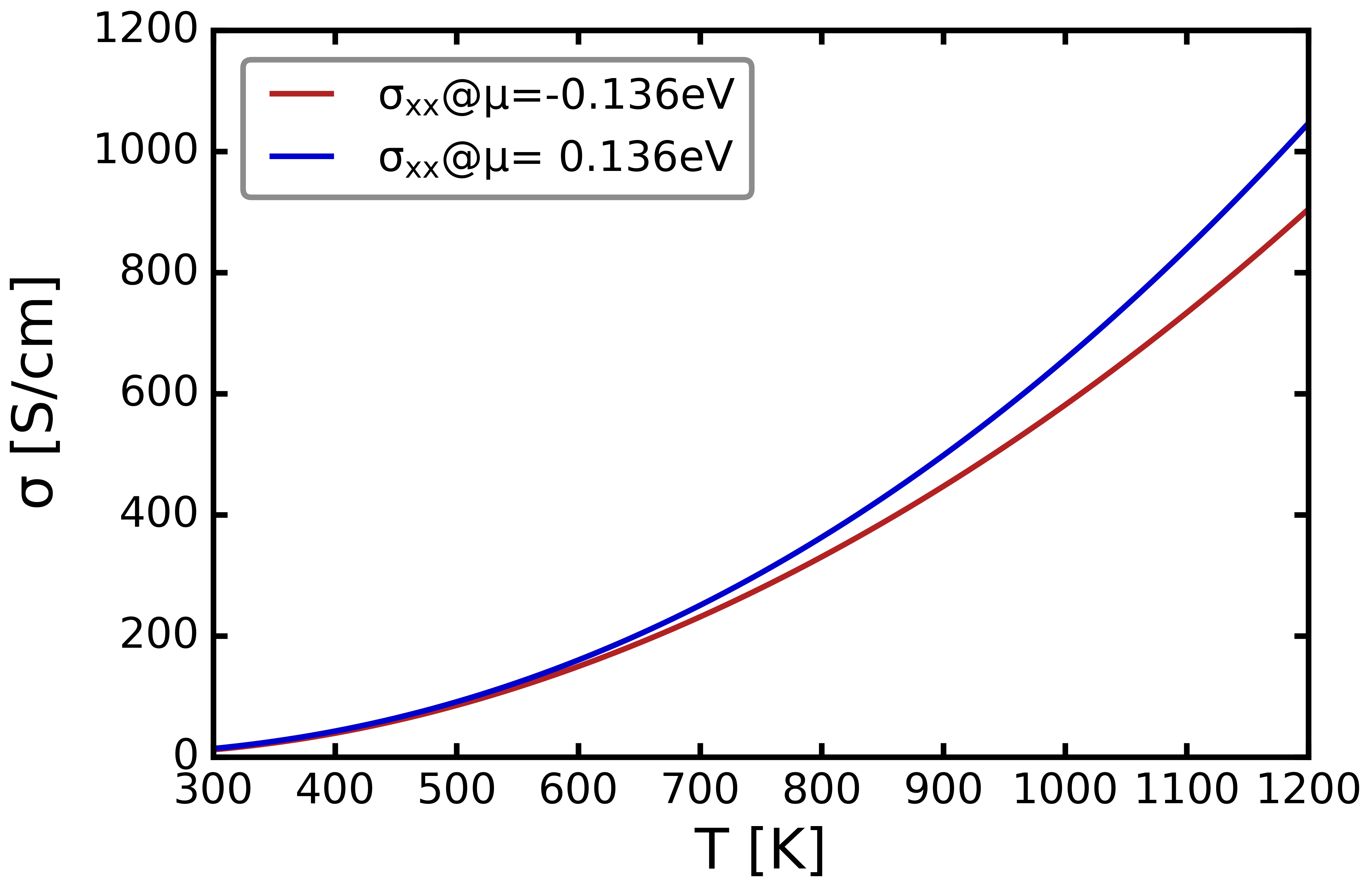
Again, using τ = 10 fs, the electrical conductivity for these μ's is obtained as:

$ grep ' -0.136' ELECTCOND_11.OUT > E11M
$ grep  ' 0.136' ELECTCOND_11.OUT > E11P
$ PLOT-files.py -f E11P E11M  -cy 3  -ll '$\sigma_{xx}$@$\mu$= 0.136eV' '$\sigma_{xx}$@$\mu$=-0.136eV'  -x 300 1200  -lx 'T [K]'  -ly '$\sigma$ [S/cm]'  -ys 1e-16  -rp

Output:

And the corresponding power factor is

$ paste ELECTCOND_11.OUT SEEBECK_11.OUT | grep ' -0.136' | awk '{ printf $1 "\t" $2 "\t" $3*$7*$7 "\n" }' > PF11M
$ paste ELECTCOND_11.OUT SEEBECK_11.OUT | grep  ' 0.136' | awk '{ printf $1 "\t" $2 "\t" $3*$7*$7 "\n" }' > PF11P
$ PLOT-files.py -f PF11P PF11M  -cy 3  -ll '${\sigma S^2}_{xx}$@$\mu$= 0.136eV' '${\sigma S^2}_{xx}$@$\mu$=-0.136eV'  -x 300 1200  -lx 'T [K]'  -ly '$\sigma S^2$ [$\mu W\,cm^{-1}\,K^{-2}$]'  -ys 1e-10  -rp

Output:

---

Bibliography

1. Method described in detail in: B. R. Nag, "Electron Transport in Compound Semiconductors" (Springer Verlag, Berlin, 1996).

2. G. D. Mahan and J. O. Sofo, "The best thermoelectric", Proc. Natl. Aad. Sci. USA 93, 7436 (1996).

3. T. J. Scheidemantel, C. Ambrosch-Draxl, T. Thonhauser, H. V. Badding, and J. O. Sofo, "Transport coefficients from first-principles calculations", Phys. Rev. B 68, 125210 (2003).

 

http://exciting.wikidot.com/oxygen-boltzmann-equation